In short
The IDE is the project’s coding environment: editor, console, terminal, and execution of R, Python and SQL. In server mode, packages are declared in a managed environment that travels with the project, so a colleague gets the same versions. In server mode code runs on the server; in browser mode it runs in your tab.
Coding where the data is
The usual arrangement keeps the tools apart: the data on one side, RStudio or Jupyter on the other, and manual exports in between that must be redone on every update.
Linkr’s IDE puts the code inside the project. Your scripts reach the datasets and databases through stable paths, they leave in the export with everything else, and they are versioned alongside the cohorts and dashboards.
This is not a replacement for RStudio
It is an integrated working environment, not a software-development IDE. For an analysis, a cleaning step, a figure, it does the job. To develop an R package, stay with your own tools.
The screen
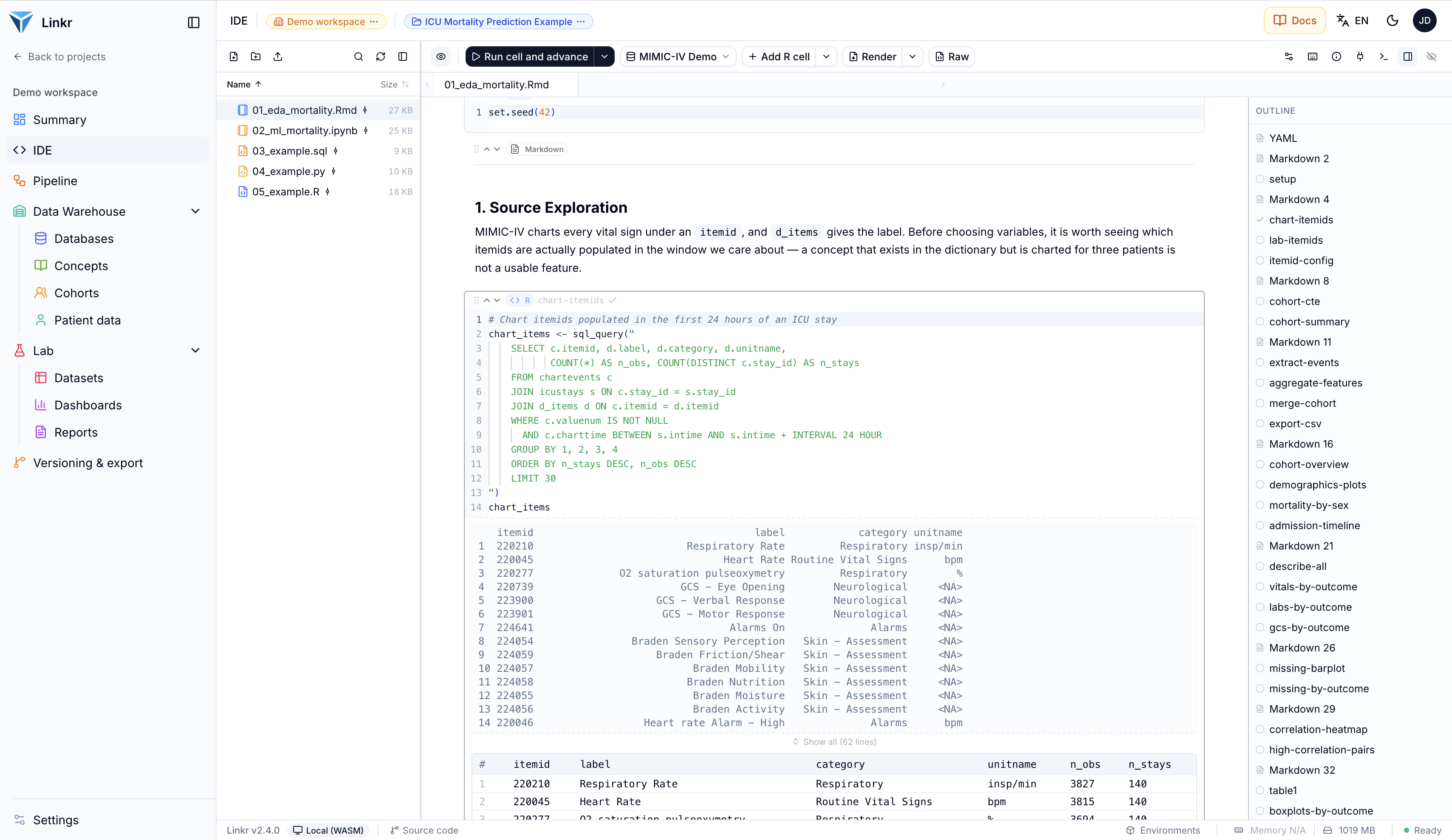
Four areas side by side: the file explorer on the left, the editor in the middle as tabs, a notebook’s outline, then the output panel on the right. The editor toolbar carries the Run button and, on the right, the settings, keyboard shortcuts, Connections, terminals, and the outline and output toggles. Below the screen, the status bar leads to background jobs and to Environments.
stays <- sql_query("SELECT * FROM visit_occurrence")nrow(stays)fit <- survfit(Surv(days, death) ~ group, stays)ggsurvplot(fit)Outline
Click the plug to open Connections.
The output panel separates result types: Console for text, plus dedicated tabs for figures, tables and HTML or markdown renders.
Terminals open as tabs in the editor, from the Terminal icon: a Bash terminal, a Python console, an R console.
Reusing output tabs
By default each run opens new tabs. The Reuse output tabs option, in the IDE settings, makes a re-run replace the script’s table and figures instead of stacking them. On a script you launch fifty times, that is a considerable comfort.
The editor’s theme, font and auto-save live in your profile, not here — they are personal preferences, not project settings.
Connections
The Connections panel says which database SQL and the sql_query() function run against. It lists two families: Warehouse databases, that is the databases linked to the project, and Custom connections, specific to the IDE, created with Add connection. Clicking a row makes it the active connection; the choice is saved with the project. The list next to the Run button makes the same choice without opening the panel.
The languages
| File | Language |
|---|---|
.py | Python |
.R | R |
.sql | SQL |
.Rmd, .qmd | R Markdown notebooks |
.ipynb | Jupyter notebooks |
Notebooks run cell by cell, with an outline on the right listing the cells and their state.
Running
The Run button runs the whole file; its arrow offers four gestures: the file, the selection, the current line, or — in server mode, and outside SQL — the file as a background job.
↑ server mode
Keyboard shortcuts are rebindable from the shortcuts window, reachable from the toolbar.
Where your code runs
This is the most important difference between the two deployment modes, and it changes what you can do.
Server mode
Real R and Python processes, on the server.
Every package on CRAN and PyPI, output appearing as the run proceeds, full terminals, and background jobs.
Browser mode
R and Python compiled for the browser.
Nothing to install, nothing leaving your machine — but a restricted package choice, output arriving all at once at the end, and no background jobs.
A terminal’s banner always says which of the two you are on.
SQL, however, does not change
A SQL query runs against the active database in both modes, with a preview capped at 1,000 rows. You simply need a connection selected, otherwise the Run button stays inactive.
Reaching the project’s data
Two libraries are available in every Linkr session, one per language. They give you the project’s paths:
import linkr
import pandas as pd

df = pd.read_csv(linkr.datasets_dir() / "cohort.csv")

con = linkr.connect("mimic")          # a database linked to the project, read-only
patients = con.sql("SELECT * FROM person LIMIT 100").df()library(linkr)
df <- read.csv(file.path(linkr_datasets_dir(), "cohort.csv"))Never derive one folder from another
Writing ”../datasets” or starting from the working directory works — until the day someone moves one of the folders in the project settings. The three locations (code, IDE, datasets) are independent and can be re-pointed separately. Always use the accessors.
These functions also work outside Linkr: run on your own machine, the same script falls back to the working directory, with a warning. A script written here therefore stays runnable elsewhere.
A CSV written to the datasets folder becomes a dataset
The folder is read straight from disk: a file a script drops there appears in Lab › Datasets, with no import step. You may need to refresh the list to see it. Note that the file must land in that folder — a CSV written beside it stays an IDE file.
Package environments
This is the mechanism that makes an analysis reproducible, and it is worth understanding. It concerns server mode; browser mode has its own rules, below.
Each project has one Python environment and one R environment. You declare your packages there; Linkr installs them in an isolated space belonging to the project. The list and exact versions are versioned with the project, in its environments/ folder.
The consequence is the one you want: a colleague importing your project rebuilds the same environment, with the same versions, and gets the same results.
Declaring packages
The Environments window opens from the status bar, at the bottom of the screen. One tab per language; you add several packages at once, comma-separated, pinning a version where needed: pandas, numpy==1.26. An environment that is still empty offers Install the workspace’s default packages: the starting set defined in the workspace settings.
Environments
Python and R run on the server in full-stack mode.
| Package | Version | Docs | Status | Actions |
|---|---|---|---|---|
| matplotlib | 3.9.2 | — | ||
| numpy | 1.26.4 | — | ||
| pandas | 2.2.3 | — | ||
| scikit-learn | 1.5.2 | — |
The environment is up to date: every declared package is installed.
A badge says where the environment stands: Not built when the list changed without being installed yet, Building… during installation, Build failed if it failed, and Up to date when everything declared is installed. Building is triggered by the Rebuild button, or automatically the first time you run code. The Rebuild automatically option applies each change immediately; turned off, changes wait for the next build.
Updating
Check for updates queries the package repository — on demand, never automatically — and fills the Status column: Up to date, or the version available. Each row has its Update to latest button, and Update all moves every package to its latest version. Either way the environment turns Not built again — or rebuilds at once if Rebuild automatically is ticked.
The Advanced options set where packages come from — the CRAN repository for R, the PyPI index for Python —, useful behind a hospital’s internal mirror. Left blank, they take the workspace’s setting.
Avoid pip install and install.packages() in a script
It works, and Linkr does not forbid it — but it warns you. A package installed that way is usable now, and until the environment is next rebuilt on this machine. It is not recorded in the versioned list: absent from the export, absent from the git repository, absent for your colleagues.
The warning offers a button to redo the installation properly inside the environment.
In browser mode packages are more limited
Installation works, and survives a page reload. But the packages belong to the browser, not the project: shared between your projects, they are neither versioned nor exported. Compiled packages — pandas, numpy — are fixed at the version the engine ships, and version pinning does not exist at all for R.
Sessions and background jobs
Several sessions
A session is an independent coding workspace, like a second console in RStudio. Useful for leaving a long computation running on one side while exploring on the other.
Each session belongs to one language: an R session only appears on an R script.
A session opened before a rebuild keeps the old environment
It goes on using the previous interpreter: packages installed since are not importable. Linkr flags this and offers to restart the session — which clears its variables.
Running as a background job
Run file as background job launches the script in a fresh process, followed from the jobs panel at the bottom of the screen. You can close the file, change page: the computation continues, and both its figures and its result table are kept.
A background job does not see your variables
It starts with an empty workspace. That is deliberate: a long computation should be reproducible, so it starts from scratch. To pass it data, write a file in the project.
Limits and permissions
Running code is Linkr’s most sensitive permission — it allows arbitrary code to run on the server. It is therefore separate from the permission to view a dashboard, and reserved for editing roles.
An administrator can disable code execution entirely on an instance.
The values below are the server-mode defaults; an administrator can adjust them.
| Limit | Default |
|---|---|
| Length of an interactive run | 2 minutes |
| Length of a background job | 30 minutes |
| Concurrent code sessions per user | 5 |
| Idle time before a session closes | 1 hour |
| Result table preview | 1,000 rows |
Going further
- Datasets — what scripts read and produce.
- Web apps — running a Shiny or Streamlit app from this code.
- Versioning and export — what leaves with your scripts.
- SQL script collections — for SQL meant to be shared.