In short
A dataset is a table ready for analysis: one row per unit of analysis — a patient, a stay — and one column per variable. You import it from a file, organize it in folders, correct it straight in the table, and attach its own analyses to it. Every change is recorded as a reversible operation: the source file is never touched.
The format analysis expects
The warehouse stores data in long format: one row per measurement, with a column saying what it is. That is the right shape for a warehouse, where you cannot know in advance which variables will exist.
Analysis expects the opposite — wide format: one row per unit of analysis, one column per variable. That is what R, Python and dashboards read. A dataset is that table.
The unit follows from the question, exactly as a cohort’s level does: one row per patient, per hospitalization, per unit stay — or per day of stay when following a trajectory. The same warehouse therefore yields datasets of very different shapes, and it is that unit which determines what a row means.
Both formats are explained in detail elsewhere
Why the difference exists, and how to move between them: Organizing your data.
Datasets live in the project’s lab, beside the dashboards — that is, on the side of what you build, never on the side of source data.
The source file is never modified
This principle governs the whole page, and it is worth understanding before touching anything.
When you correct a cell, add a row or delete a column, Linkr does not write to your file. It records your action in a log, and replays that log over the original file each time it is displayed.
The imported file
Immutable.
Your CSV, Excel or Parquet, exactly as you dropped it in. Nothing is ever written to it.
The operation log
Your corrections, in order.
”this cell now holds this value”, “this column is deleted”. Each one can be undone.
Three practical consequences:
- Nothing is irreversible. The Discard all changes button returns to the original file, however many corrections you made.
- Your corrections are inspectable. The Edit history lists them most recent first, in plain words: “Column weight added (number)”, “Row 42 deleted”.
- You can account for everything. If someone asks why a value differs from the patient record, the answer is in the history.
Editing is off by default
A dataset opens read-only. The Edit data button turns editing on, and that state belongs to the dataset it was turned on for: switching files puts you back in read-only, with no risk of correcting the wrong table by accident.
Creating a dataset
Several routes, depending on where your data comes from.
Import a file
The common case. CSV, TSV, Excel or Parquet, dragged in or picked from disk.
From a script
An R or Python script in the IDE that writes a CSV into the datasets folder sees it appear here automatically.
Create an empty table
For manual entry: you declare the columns, then fill them in. Useful for collecting data on a few dozen patients.
To which add duplicating an existing dataset, and datasets arriving with an imported project.
Importing a file
The import dialog shows a preview of the first ten rows before you confirm anything — that is where reading errors are caught.
It offers an import preset based on where the file came from:
| Preset | What it does |
|---|---|
| Plain table | One row per record, one column per field. No questionnaire structure. |
| Goupile (eCRF) | Joins every form sheet on the record id, and takes its labels from the form dictionary. |
| REDCap | Reads a REDCap export; its data dictionary supplies the questions, choices and branching. |
| XLSForm / ODK | Reads an ODK, KoboToolbox or SurveyCTO export. Multiple-choice answers become one column per option. |
Linkr detects the preset from the file — a workbook exported from Goupile, for instance — and marks it Detected from the file; you can change it.
Upload dataset
Upload a CSV, Excel, or Parquet file to create a new dataset.
admissions.csv
1 284 rows · 5 columns
Import preset
One row per record, one column per field. No questionnaire structure.
Delimiter
Encoding
Skip rows
Header row
Tokens read as empty. A numeric column containing these still counts as a number.
| # | stay_id | age | sex | saps2 | admitted_on |
|---|---|---|---|---|---|
| 1 | S-1042 | 67 | 1 | 41 | 2024-03-02 |
| 2 | S-1043 | 54 | 2 | 28 | 2024-03-02 |
| 3 | S-1044 | 81 | 1 | null | 2024-03-04 |
| 4 | S-1045 | 73 | 2 | 52 | 2024-03-05 |
For a CSV you adjust the delimiter, the encoding, how many rows to skip and whether there is a header row; for an Excel file, the sheet to read. Each setting re-reads the file and refreshes the preview: a wrong delimiter shows at once, every value squeezed into a single column. Each header carries its detected type; clicking the badge forces it, and a ring flags a forced type.
Declare your missing values
The Missing values field lists the tokens to read as empty: by default na, n/a, null, nan, none, #n/a. This is what lets a column stay numeric despite a few NA cells. The hyphen and the full stop are deliberately absent: they are legitimate values too often.
Getting the options wrong does not mean starting over
The original file is kept. Right-click the dataset, then Import settings, to change the delimiter or the encoding and re-read the file — no manual re-import needed.
Working on a dataset
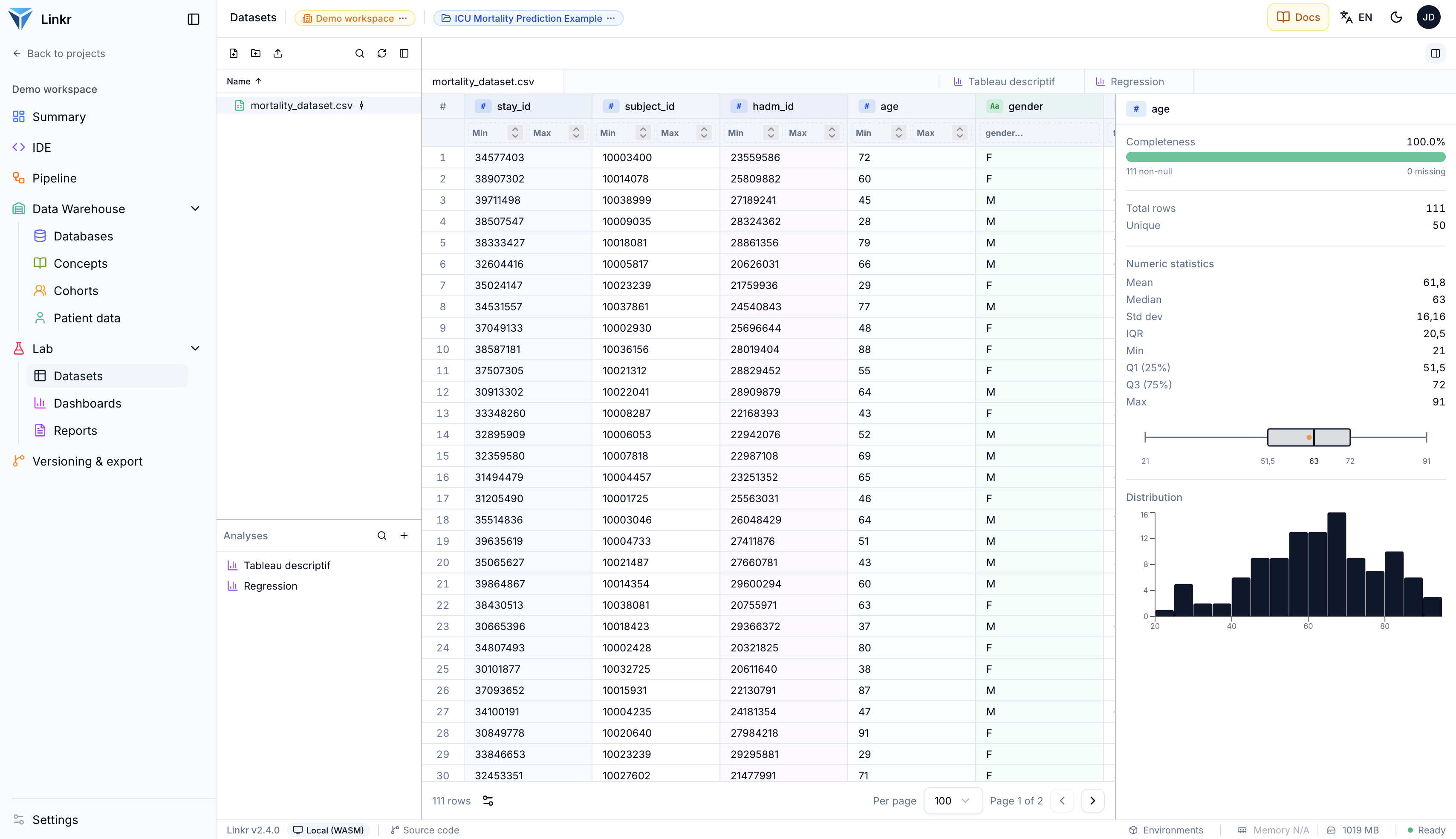
The screen is laid out like an editor, in four zones: on the left, the dataset tree and, below it, the analyses panel of the selected dataset; in the middle, the table — or the open analysis, in a tab next to the file; on the right, the column statistics, which step aside when an analysis is in front.
Datasets are arranged in folders — useful as soon as a project holds a dozen of them.
Columns
A column header’s menu offers sorting, pinning, hiding and moving, plus two entries worth a word.
Treat as forces a column’s type: a column of codes read as numbers becomes text again, and leading zeros stop disappearing.
Edit label & description separates two things often conflated:
- the name is technical — the file’s header, the one you write in a script;
- the label is what appears on screen, and it can be translated.
You can also declare value labels: 1 becomes Male, 2 becomes Female, in tables and charts alike, without the data changing.
Edit column
Add a friendly label and description for “sex”. The technical name stays unchanged.
Label
Description
Value labels
Give each stored code a readable label. Stored data is unchanged — labels are only shown in tables, charts and filters.
12In the table
Renaming a column does not break your dashboards
A column’s internal identifier derives from its name, so renaming changes that key. Linkr repairs the chain in the same action — filters and widgets follow. Only one situation is refused: if the new name would collide with an existing column, the rename is blocked rather than silently pointing your widgets at the wrong column.
Re-importing the same file preserves your dashboards
Column identifiers are derived from names, identically in browser and on the server. An updated file, re-imported, produces the same identifiers: your filters and widgets stay attached. Note that accents and punctuation are normalized away, so Âge and age name the same column.
Correcting data
The Edit data button sits under the table. Once it is on, a click selects a cell and you edit it as in a spreadsheet: double-click, or Enter, or just start typing. Enter confirms and moves down one row. The Row button inserts a row above or below the selection, or at the end; Column adds one. Right-clicking a row number moves or deletes that row.
| # | Aastay_id | #age | Aasex | #weight_kg | ventilated |
|---|---|---|---|---|---|
| 1 | S-1042 | 67 | M | 81 | true |
| 2 | S-1043 | 54 | F | 63 | false |
| 3 | S-1044 | 81 | M | 7.4 | true |
| 4 | S-1045 | 73 | F | null | true |
| 5 | S-1046 | 412 | M | 92 | false |
Next to them, Undo removes the last operation, and the counter opens the Edit history. It lists each operation with its author and date, and offers three actions: Compact, which merges redundant operations — ten successive corrections of one cell become one —, Undo last change, and Discard all changes, which returns to the source file after confirmation.
Constraining entry
For a dataset filled in by hand, the Edit column dialog accepts constraints: required, allowed values (a dropdown rather than a free field), minimum and maximum, and include time of day for a date.
These constraints apply to entry, not to imports
They guide what is typed into Linkr. They do not retroactively reject data already imported: setting a maximum of 120 on an age will not surface outliers in an existing file. To check imported data, see Data quality.
Column statistics
For the selected column, the right-hand panel shows the row count, missing values, unique values and completeness — then, depending on the type, mean, median, standard deviation and distribution, or the time span covered.
This is the reflex to have after an import: 40% completeness on a variable expected everywhere usually signals a reading problem, not a data problem.
Analyses
An analysis is a treatment attached to a dataset: a Table 1, a key indicator, a chart, a survival curve — or your own R or Python code. It sits in the Analyses panel, under the tree, and opens in a tab next to the file.
| # | Aastay_id | #age | #saps2 |
|---|---|---|---|
| 1 | S-1042 | 67 | 41 |
| 2 | S-1043 | 54 | 28 |
| 3 | S-1044 | 81 | null |
| 4 | S-1045 | 73 | 52 |
| 5 | S-1046 | 41 | 19 |
| 6 | S-1047 | 69 | 37 |
Column statistics
#age
The + of the panel opens New analysis: a name, then a Plugin or Custom code. The plugins are the dashboards’ ones — see Built-in widgets and Analysis widgets. A plugin with settings opens a second screen: the configuration on the left, a live preview on the right, and its documentation in the Doc tab. Custom code opens a Python or R editor on the dataset.
An open analysis is set up from its Config panel, and Save keeps its configuration. Its result exports as PNG, and a table copies as is or as LaTeX.
An analysis follows its dataset
It is attached to one file: selecting another dataset shows that one’s analyses. On export, analyses leave with the dataset’s structure, in its folder — even when its rows stay on the machine.
Where the data lives
Storage differs with your installation, which explains a few behavioural differences.
Browser mode
Everything stays in your browser.
Rows are held in memory. The limit is your machine’s — a few hundred thousand rows are fine, several million are not.
Server mode
Files live on the server.
The table pulls down one page at a time, which allows far larger volumes. A Refresh button re-reads the folder if files were placed there outside Linkr.
Editing works the same way in both, and the source file stays intact either way.
What goes into an export
A dataset can be large, and can contain patient-level data. It is therefore excluded from versioning by default: what travels is the structure — columns, types, labels — not the rows.
To include a specific file, you mark it explicitly: right-click, Mark for versioning. A small commit icon then flags it in the tree. Its edit journal leaves with it — for a hand-filled collection, that is what holds the values.
Marking a dataset sends it to the git repository
Marking is decided file by file, deliberately. Before marking, check what the file holds: patient-level data pushed to a shared repository does not come back out. See Versioning and export.
Going further
- Dashboards — visualizing a dataset.
- IDE — analyzing it in R or Python.
- Versioning and export — what leaves the project, and what stays.
- Organizing your data — long and wide format.