Using the Console

Introduction

Using the Console

The Console page is accessible from any page in the application by clicking the corresponding link at the top of the screen.

You arrive at a page with:

• The choice of programming language and output
• A code editor
• A block where the result of code execution will be displayed

Start by choosing the programming language and output to use.

We’ll begin by looking at the different outputs available in R:

• Console: the displayed result will be what would be shown in the R console
• Figure: corresponds to a figureOutput from Shiny
• Table: corresponds to a tableOutput from Shiny
• DataTable: corresponds to a DT::DTOutput from DT and Shiny
• UI (HTML): the result will be displayed in a uiOutput from Shiny
• RMarkdown: corresponds to the HTML output from converting the RMarkdown file presented in the console

We’ll look at the outputs with examples. For this, load the LinkR Demo project to load the MIMIC-IV data.

R - Console

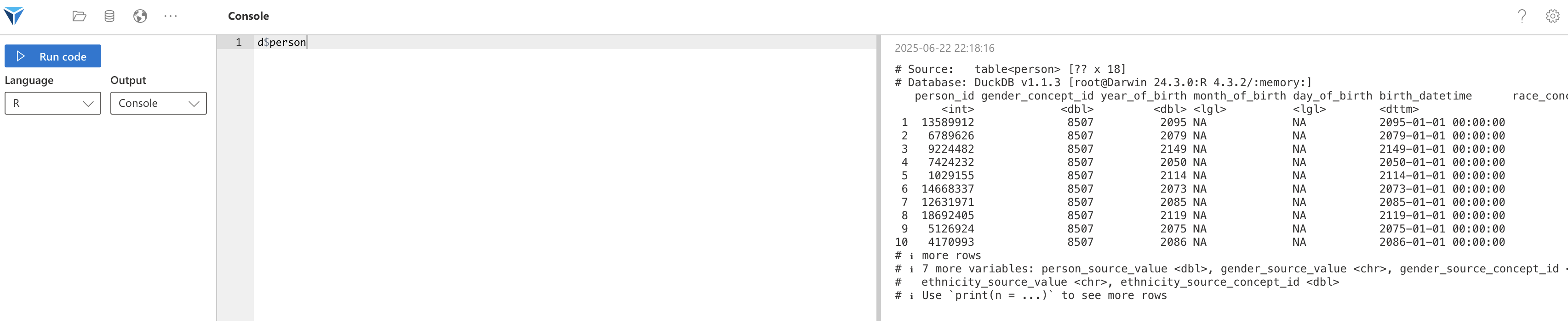
Select the “Console” output, write d$person in the text editor and execute the code (with the Execute button or with the shortcut).

R - Figure

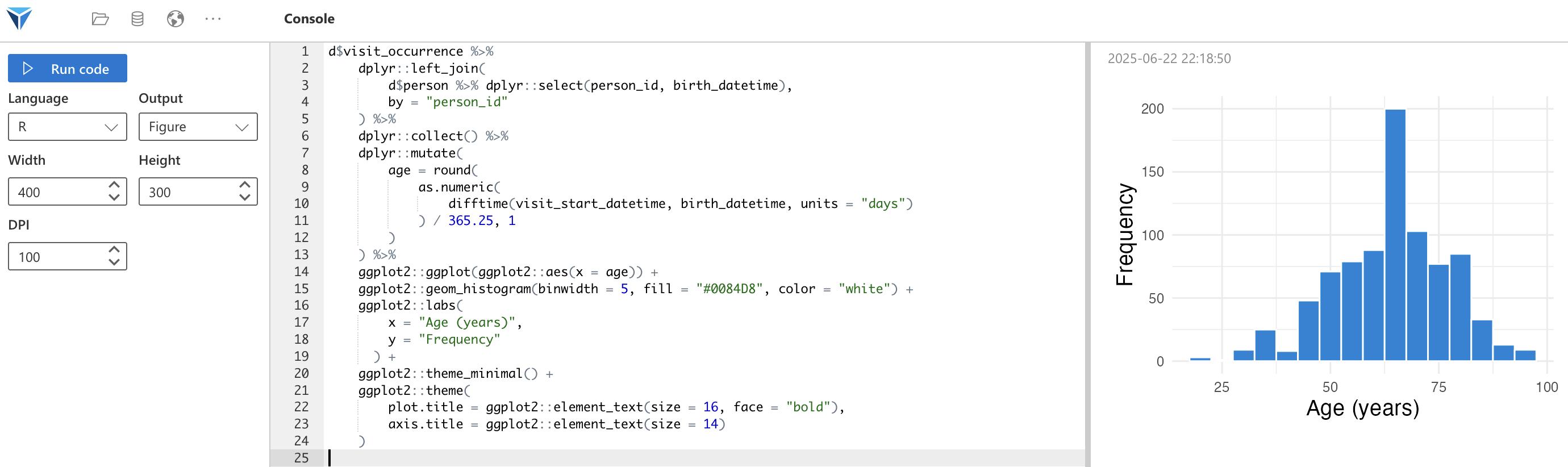
Here’s an example for creating a histogram showing patient ages from the dataset associated with the project.

Select the “Figure” output and execute this code. Note that you can configure the dimensions and resolution of the image.

d$visit_occurrence %>%
    dplyr::left_join(
        d$person %>% dplyr::select(person_id, birth_datetime),
        by = "person_id"
    ) %>%
    dplyr::collect() %>%
    dplyr::mutate(
        age = round(
            as.numeric(
                difftime(visit_start_datetime, birth_datetime, units = "days")
            ) / 365.25, 1
        )
    ) %>%
    ggplot2::ggplot(ggplot2::aes(x = age)) +
    ggplot2::geom_histogram(binwidth = 5, fill = "#0084D8", color = "white") +
    ggplot2::labs(
        x = "Age (years)",
        y = "Frequency"
      ) +
    ggplot2::theme_minimal() +
    ggplot2::theme(
        plot.title = ggplot2::element_text(size = 16, face = "bold"),
        axis.title = ggplot2::element_text(size = 14)
    )

R - Table

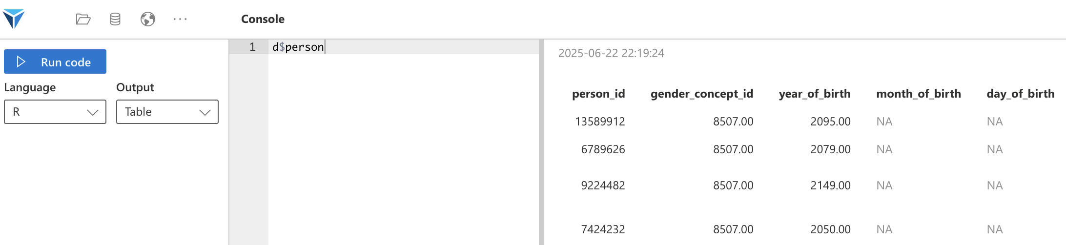
The “Table” output displays the entire dataframe using Shiny’s tableOutput function.

R - DataTable

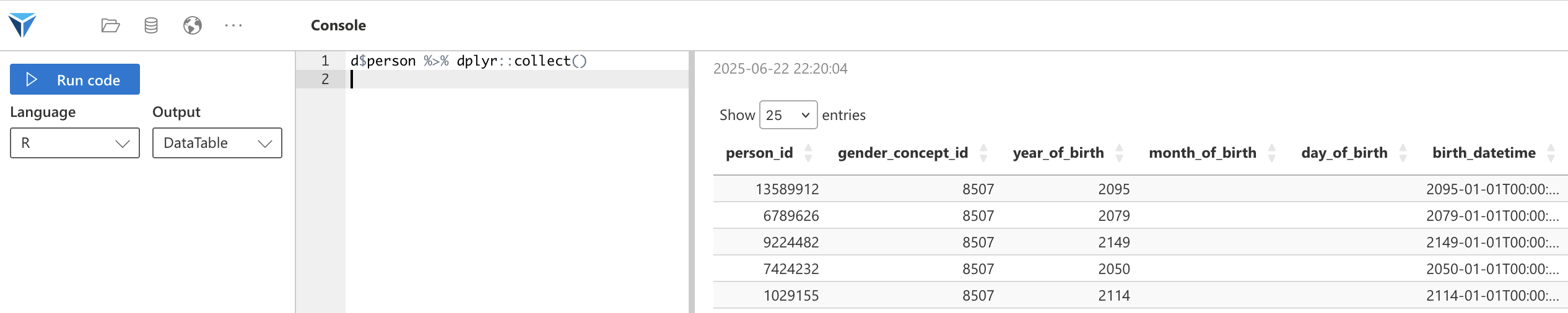
The “DataTable” output uses the DT library to display results, which provides better display than “Table” with a pagination system.

Note that data must be in memory to be displayed.

You’ll need to write:

d$person %>% dplyr::collect()

R - RMarkdown

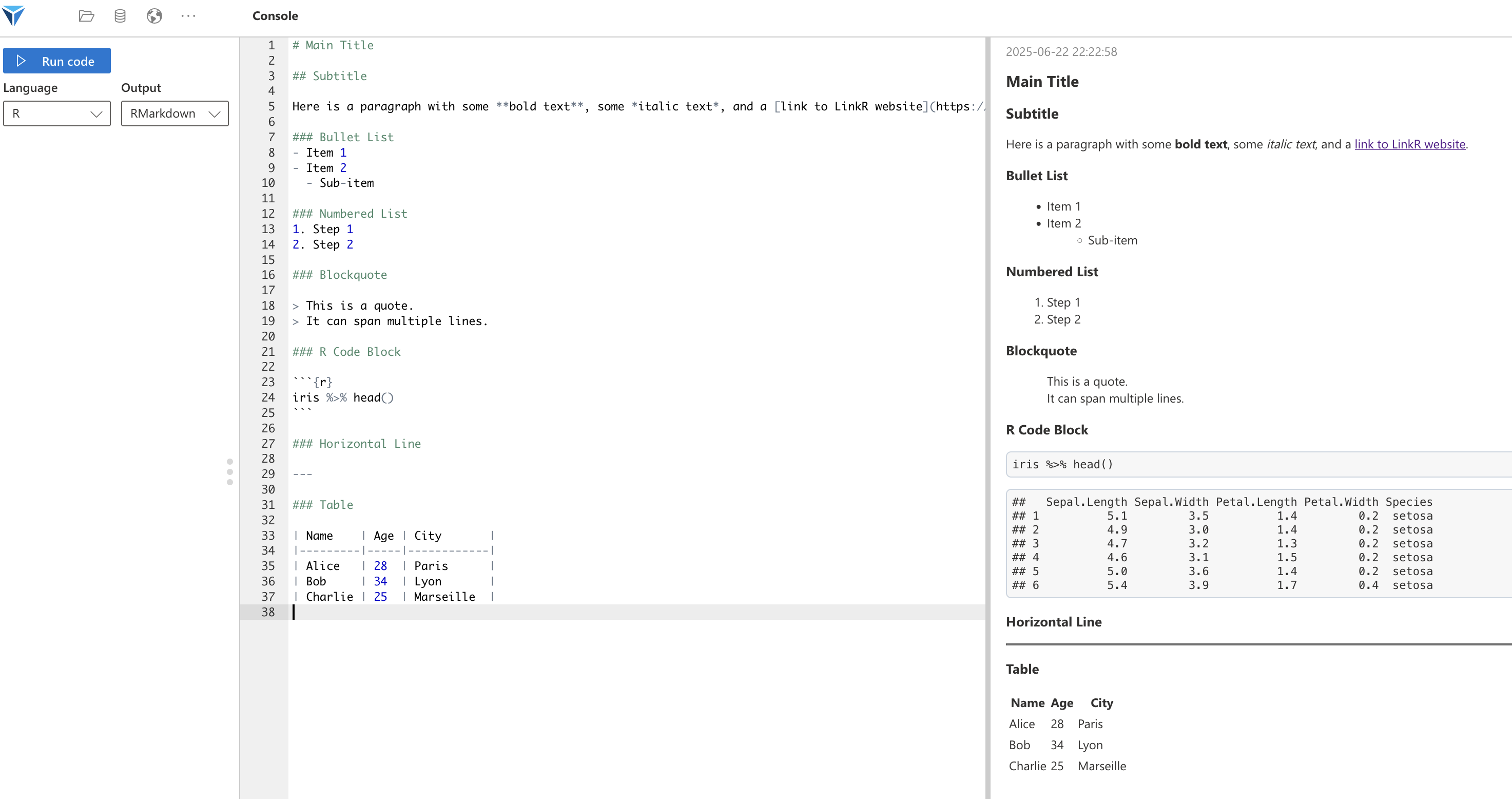
The “RMarkdown” output interprets the code as a .Rmd file.

The Markdown will be converted to HTML and the R code will be interpreted.

Python - Console

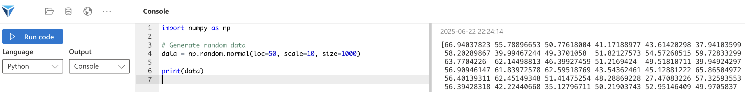
A simple example of using the console in Python:

import numpy as np

# Generate random data
data = np.random.normal(loc=50, scale=10, size=1000)

print(data)

Python - Matplotlib

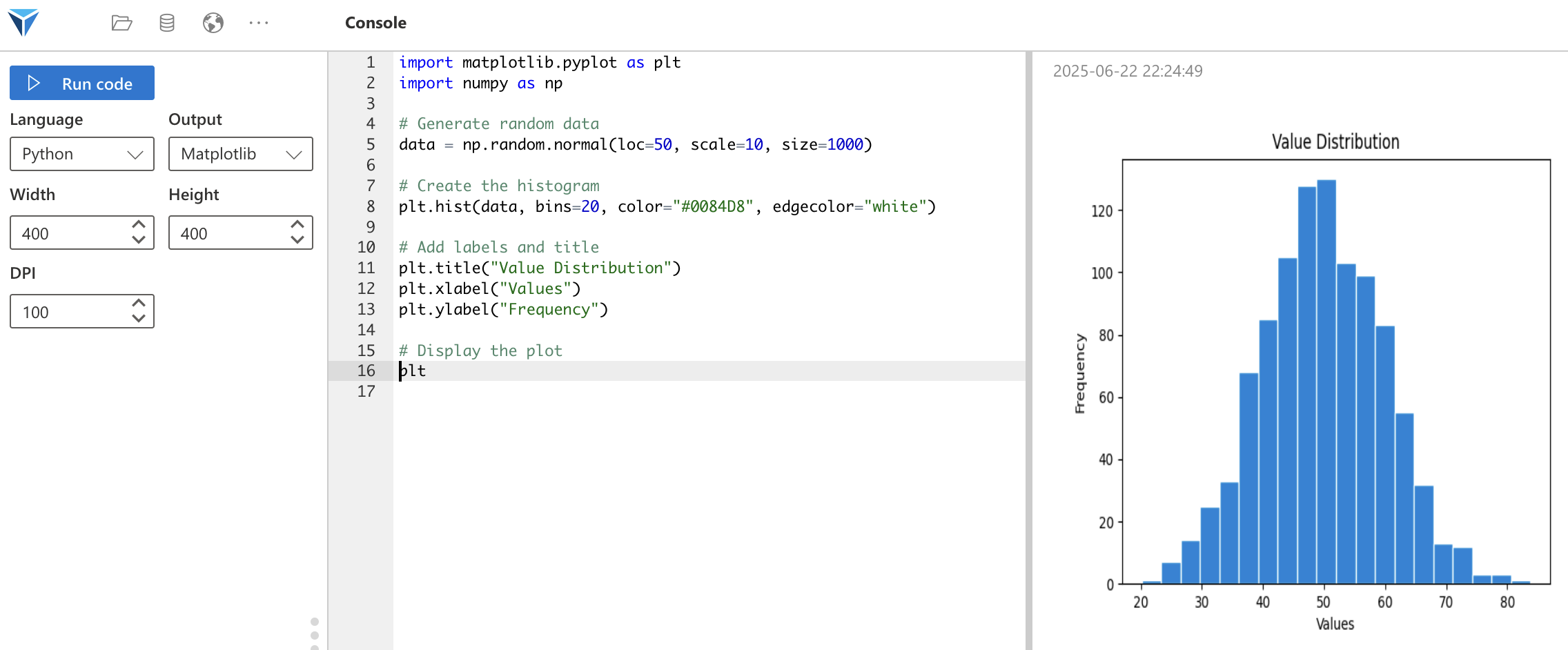
It’s also possible to use the Matplotlib library to create figures:

import matplotlib.pyplot as plt
import numpy as np

# Generate random data
data = np.random.normal(loc=50, scale=10, size=1000)

# Create the histogram
plt.hist(data, bins=20, color="#0084D8", edgecolor="white")

# Add labels and title
plt.title("Value Distribution")
plt.xlabel("Values")
plt.ylabel("Frequency")

# Display the plot
plt

Querying OMOP Data

Once data is loaded (by loading a project associated with a dataset or by loading a dataset directly), the data becomes accessible from the console through two methods:

• Through R variables prefixed with d$ (d for data)
• Through SQL queries using the R function get_query

All OMOP tables are available through both methods.

R Variables

We’ve seen in the examples above the use of variables prefixed with d$ (d$person, d$measurement, etc).

This data is loaded in lazy format, which means it’s not loaded into memory (allowing quick display of the variable even if it contains billions of rows). Once filtering operations are performed, it’s possible to collect this data into memory with the dplyr::collect() function.

In the following example, we filter data from the Measurement table on person_id 2562658 and on measurement_concept_id 3027018 (corresponding to the LOINC concept - Heart rate).

d$measurement %>%
    dplyr::filter(
        person_id == 2562658,
        measurement_concept_id == 3027018
    ) %>%
    dplyr::collect()

Note that these tables are also available for the selected patient group (or subset), with the d$data_subset list.

This will display the list of patients in the selected group:

d$data_subset$person

SQL Queries

For interoperability purposes, it’s necessary to be able to query OMOP tables in SQL.

When you import data into LinkR, it’s always a database connection (even when you import SQL or Parquet files, which are read as a DuckDB connection).

It’s possible to query data in SQL via the R function get_query.

This code allows you to display all data from the patient table:

get_query("SELECT * FROM person")

You can also use SQL queries from the tutorial usual OMOP queries.

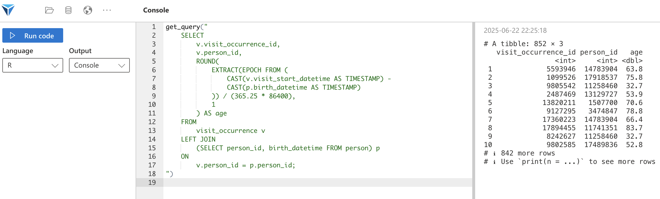
This query, extracted from this tutorial, allows you to get patient ages:

get_query("
    SELECT 
        v.visit_occurrence_id,
        v.person_id,
        ROUND(
            EXTRACT(EPOCH FROM (
                CAST(v.visit_start_datetime AS TIMESTAMP) - 
                CAST(p.birth_datetime AS TIMESTAMP)
            )) / (365.25 * 86400), 
            1
        ) AS age
    FROM 
        visit_occurrence v
    LEFT JOIN 
        (SELECT person_id, birth_datetime FROM person) p
    ON 
        v.person_id = p.person_id;
")

Querying Other Variables

Other variables, prefixed with m$, can be queried from the console. These variables are intended to be used in plugins.

Here’s the list:

• m$selected_subset: displays the ID of the patient group selected via the dropdown menu
• m$selected_person: ID of the patient selected via the dropdown menu
• m$selected_visit_detail: ID of the hospital stay selected via the dropdown menu
• m$subsets: list of patient groups available for the open project
• m$subset_persons: list of patients belonging to the selected patient group (subset)

Conclusion